Chapter 9: Random variables

STAT 1010 - Fall 2022

Learning outcomes

By the end of this lesson you should:

Know how to find the mean given a probability mass or distribution function
Understand how to use multiplication and addition rules to find expected values and variance of new random variables

Revision - 1

Find the mean, and variance for these examples:

$20, 24, 25, 36, 25, 22, 23$
Rolling a fair six-sided die

Revision - 2

A stock prices ($X$) at these frequencies:

$x$	$n$
1.23	3
1.29	5
1.37	4
1.84	1
1.18	6
1.22	2
1.25	4
Total	25

Using proportions

$x$	$n$	$P(X) = x$
1.23	3
1.29	5
1.37	4
1.84	1
1.18	6
1.22	2
1.25	4
Total	25

Mean or expected value

If we know $P(X) = x$, then we can use this to find the mean or expected value of a random variable. The pdf includes information about both the total and the number of occurrences of $x$, it does the computation for us.

$\mu = E(X)$

$= x_1p(x_1) + x_2p(x_2) + … + x_np(x_n)$

Probability density function

There are different ways to define a pdf:

table
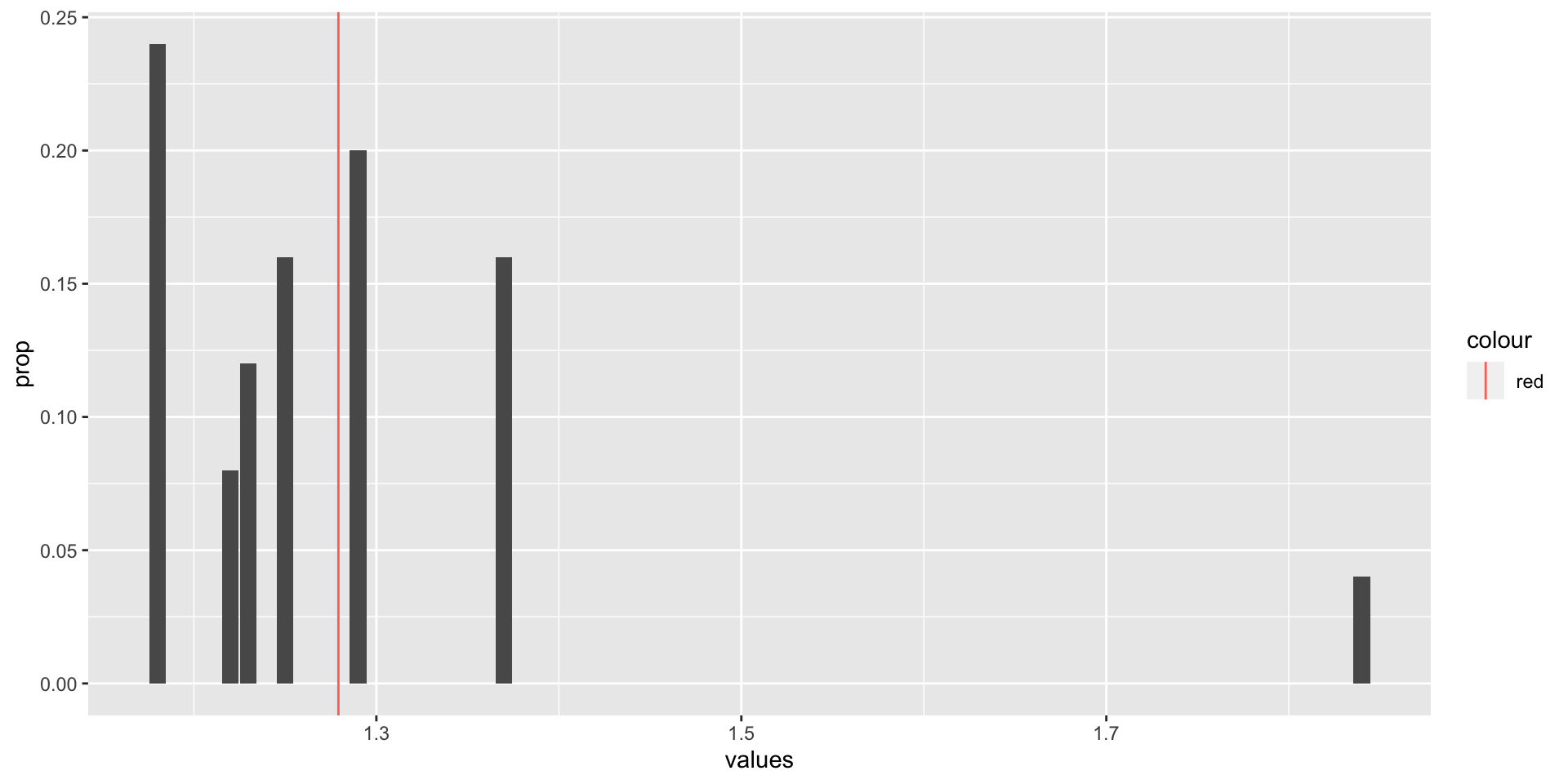
plot

plot - pdf

## Input data
values <- c(1.23, 1.29, 1.37, 1.84, 1.18, 1.22, 1.25)
counts <- c(3, 5, 4, 1, 6, 2, 4)

d <- 
  as_tibble(data.frame(values, counts)) %>% # make tibble
  mutate(prop = counts/sum(counts), # find proportion
         part_mean = values*prop,  # multiply values & prop
         mean = sum(part_mean)) # find the sum

d %>% 
  ggplot(aes(x = values, y = prop)) + # for values and prop
  geom_bar(stat = "identity") + # make bar chart of identity (prop)
  geom_vline(aes(xintercept = mean, color = "red")) # and line of mean

Price increase

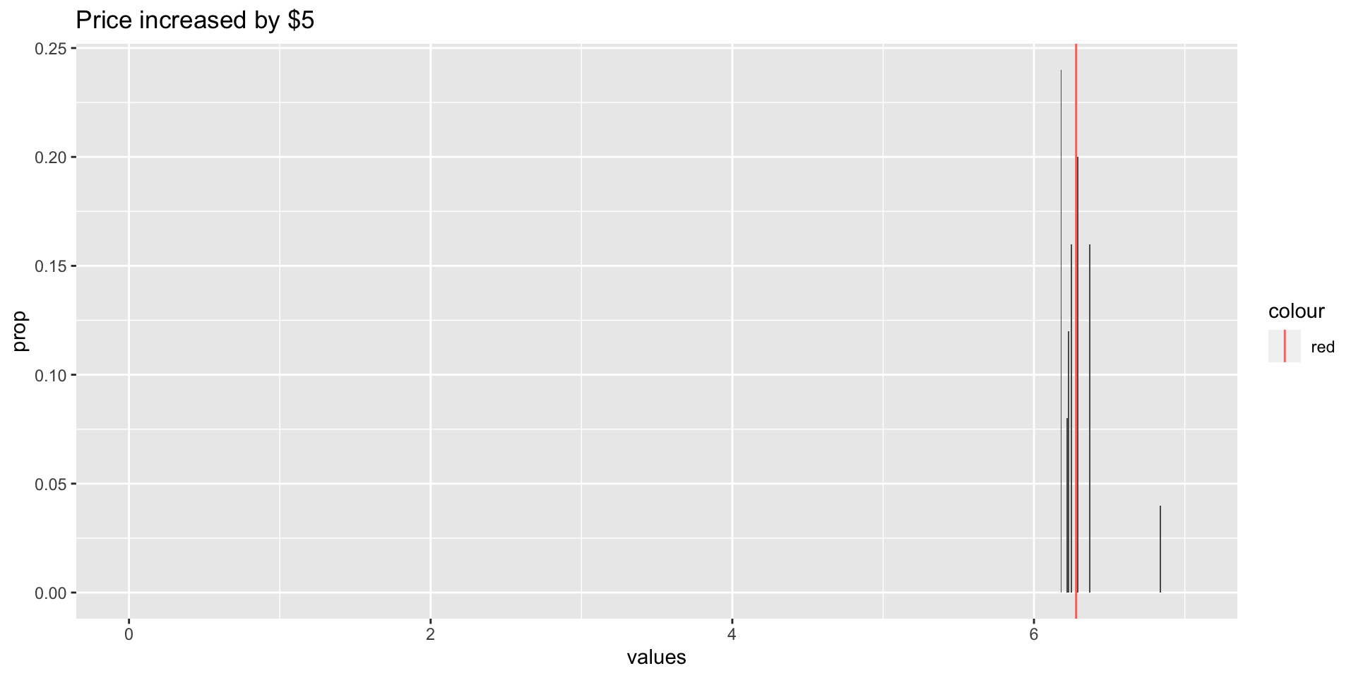
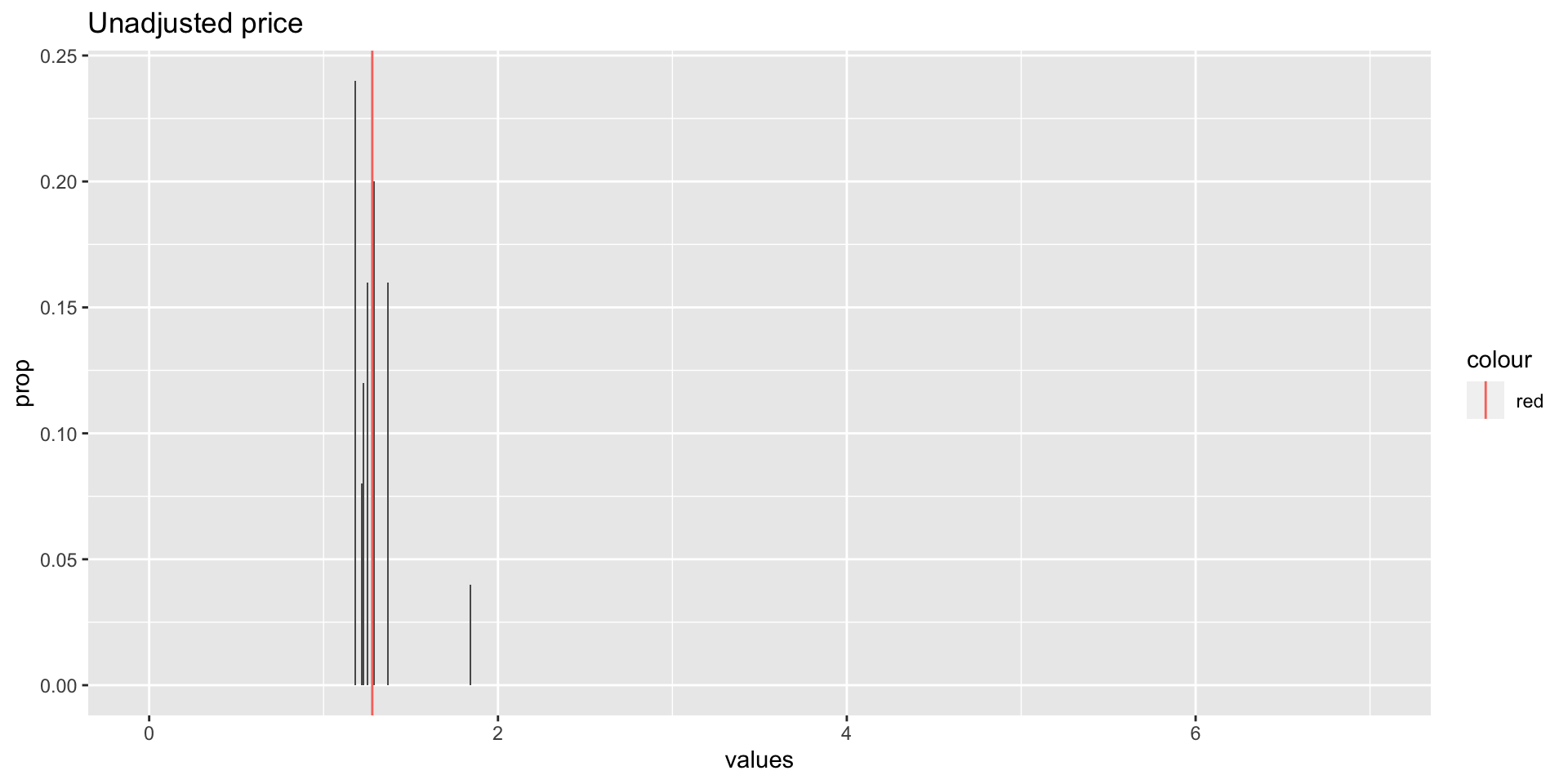
All the stock values have increased by $5:

What happens to the mean?

What happens to the standard deviation?

Price increase

$x$	$x + 5$	$P(X) = x+5$
1.23	6.23	0.12
1.29	6.29	0.20
1.37	6.37	0.16
1.84	6.84	0.04
1.18	6.18	0.24
1.22	6.22	0.08
1.25	6.25	0.16

Price increase

Adding a constant

$E(X \pm c) = E(X) \pm c$

$SD(X \pm c) = SD(X)$

$Var(X \pm c) = Var(X)$

Stock splits

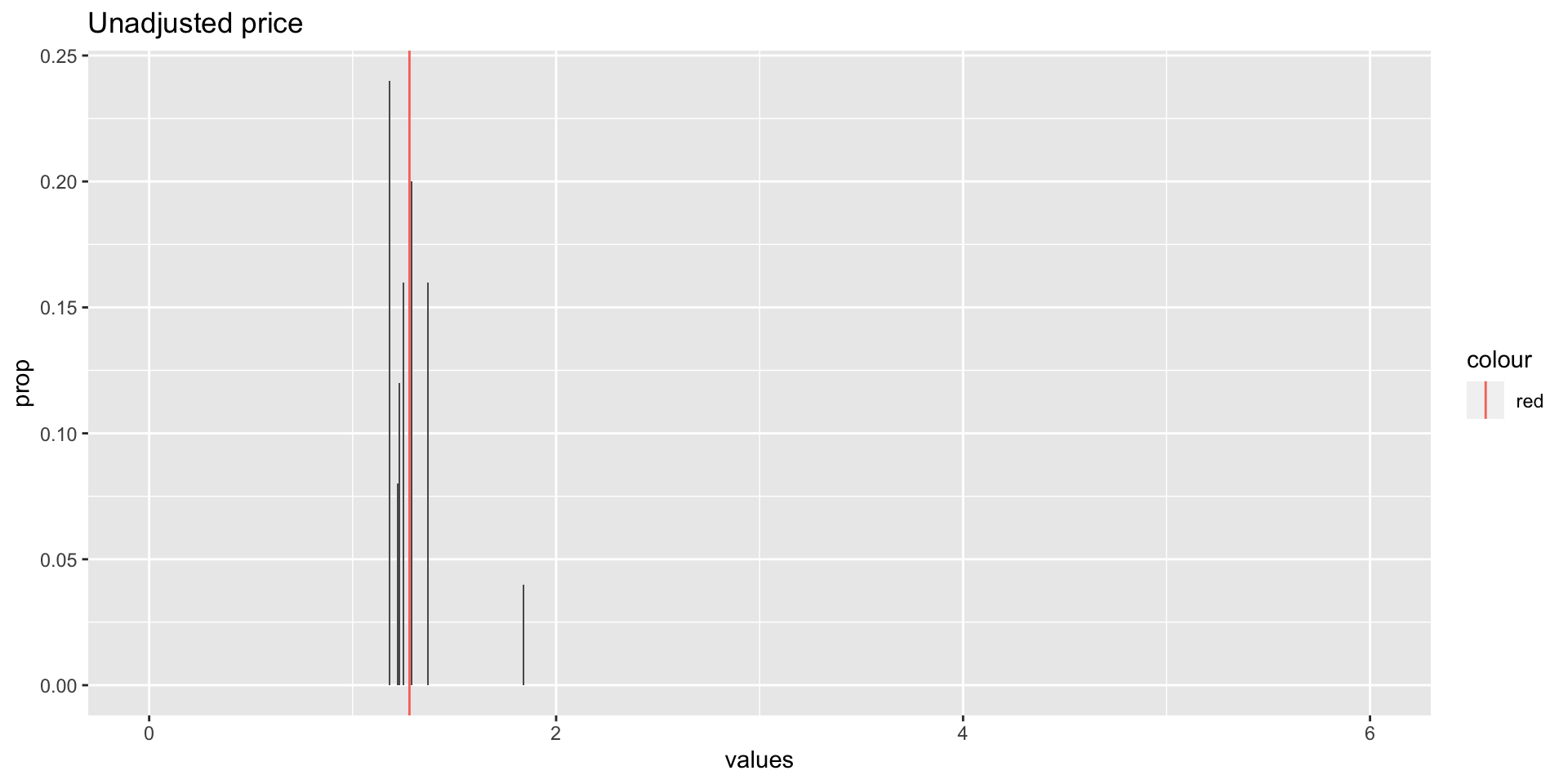
Without decreasing the cost, the stock values are now 3 times what they were before:

What happens to the mean?

What happens to the standard deviation?

Stock splits

$x$	$3x$	$P(X) = x$
1.23	3.68	0.12
1.29	3.87	0.20
1.37	4.11	0.16
1.84	5.52	0.04
1.18	3.54	0.24
1.22	3.66	0.08
1.25	3.75	0.16

Stock splits

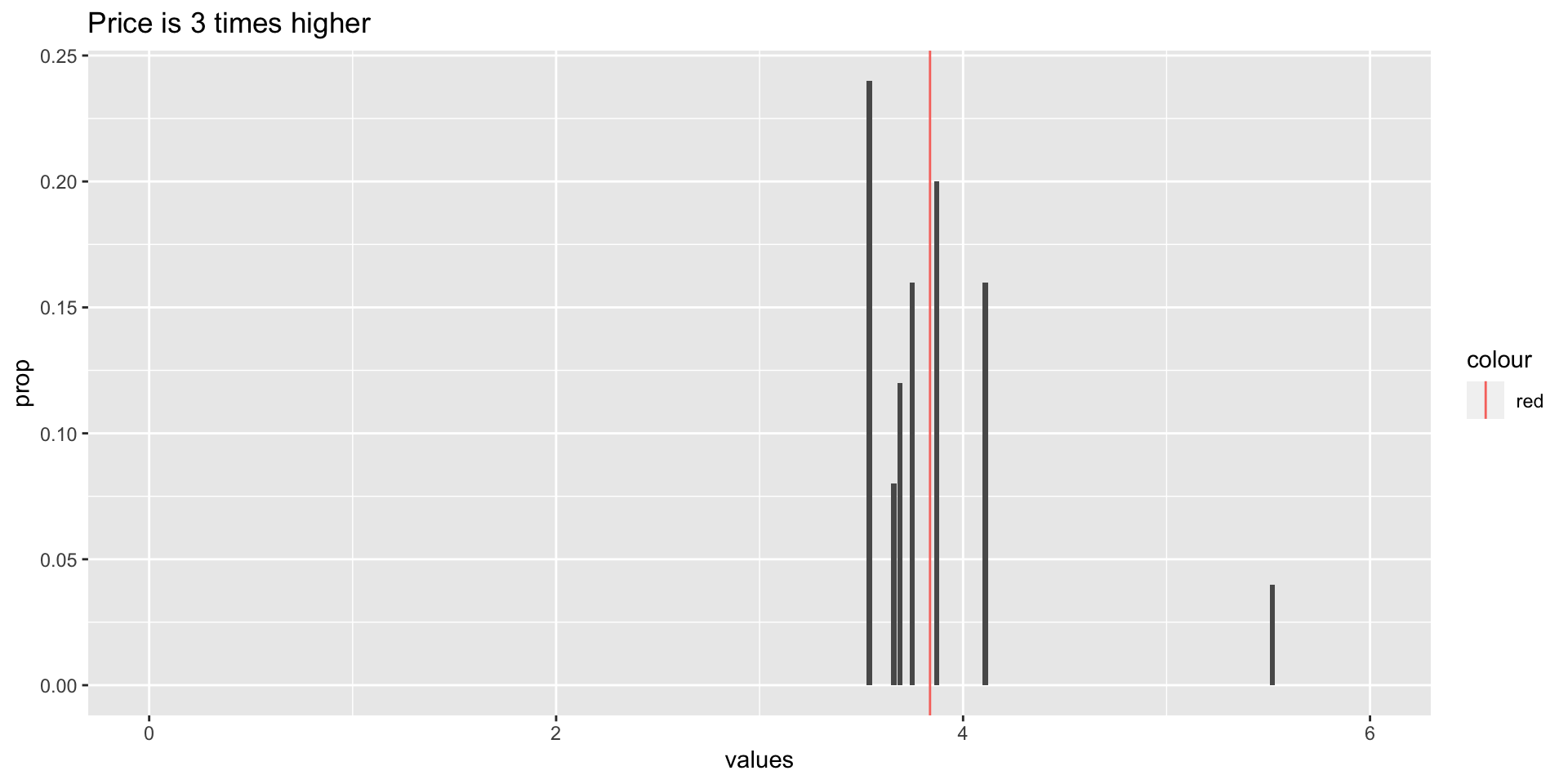
Multiply by a constant

$E(cX) = cE(X)$

$SD(cX) = |c|SD(X)$

$Var(cX) = c^2Var(X)$

$E(cX \pm a)=cE(X) \pm a$

$Var(cX \pm a)=c^2Var(X)$

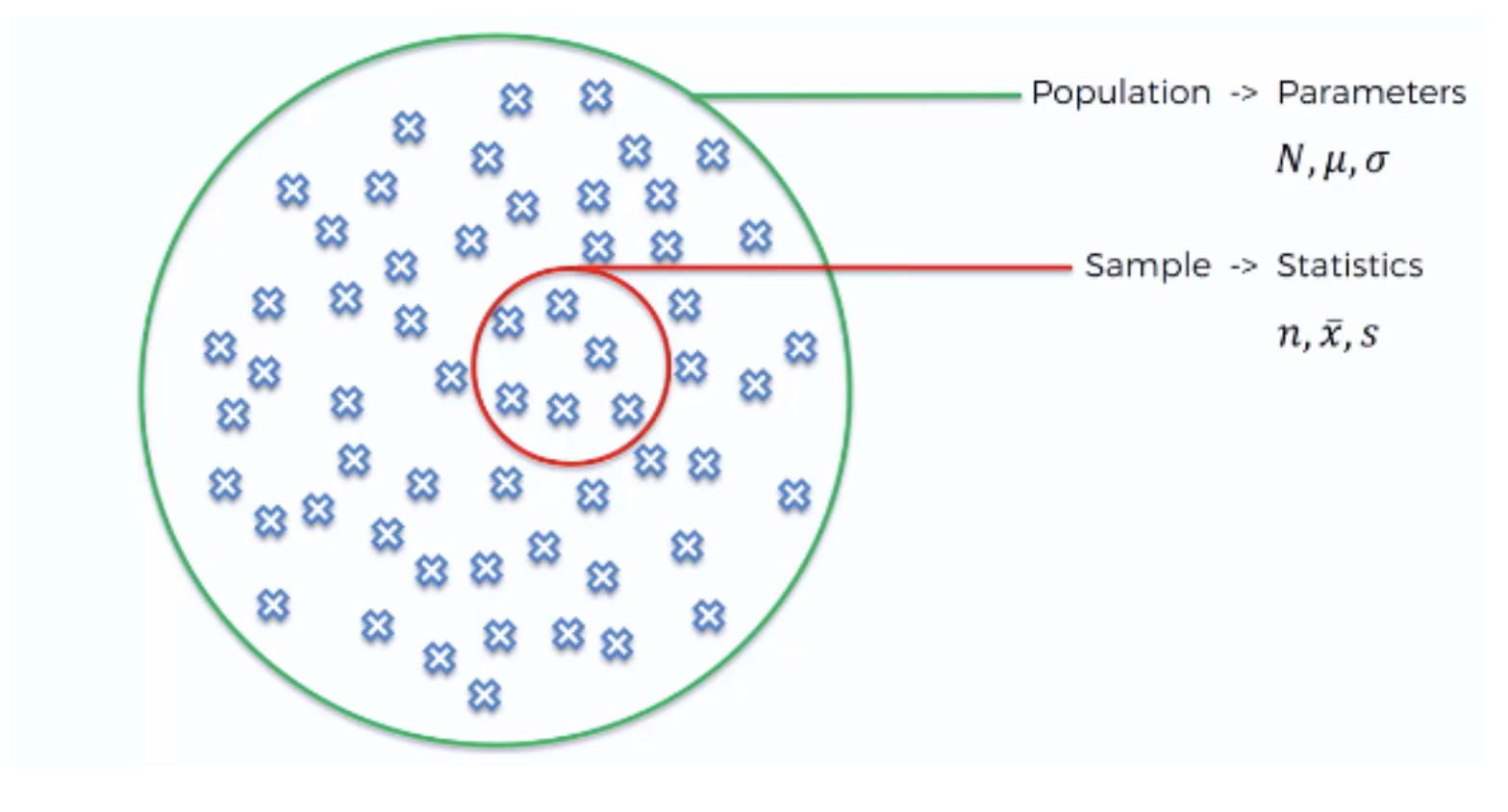
Parameter vs estimate

	population	sample
name	parameter	estimate
mean	$\mu$	$\bar{x}$
variance	$\sigma^2$	$s^2$
standard deviation	$\sigma$	$s$
size	$N$	$n$

Visually

Your turn

Click here or the qr code below