Chapter 6: Association between quantitative variables

STAT 1010 - Fall 2022

Learning outcomes

By the end of this lesson you should:

• Perform a visual association test

• Know how to read a scatterplot to describe associations between quantitative variables

• Know how to quantify associations in quantitative variables

• Use a line to describe associations in linear relationships

• Understand spurious correlations and lurking variables

Associations

When have we used this word before?

Remind them of \(\chi^2\) tests

• \(\chi^2\) tests are used for associations in categorical data
• What is used to find associations in numeric data?

Plots

Remind them about plots of proportions that we did for titanic and comics data. What did we look for in the plots?

Which variable goes on the y axis? Which on the x axis?

• variable on the \(y\) axis
  • dependent
  • response
  • outcome
• variable on the \(x\) axis
  • independent
  • explanatory
  • predictor

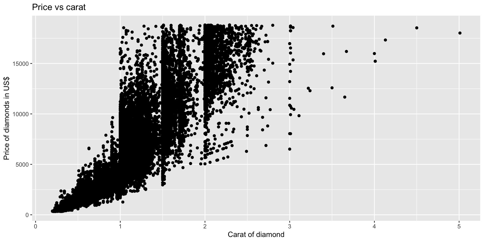
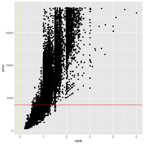
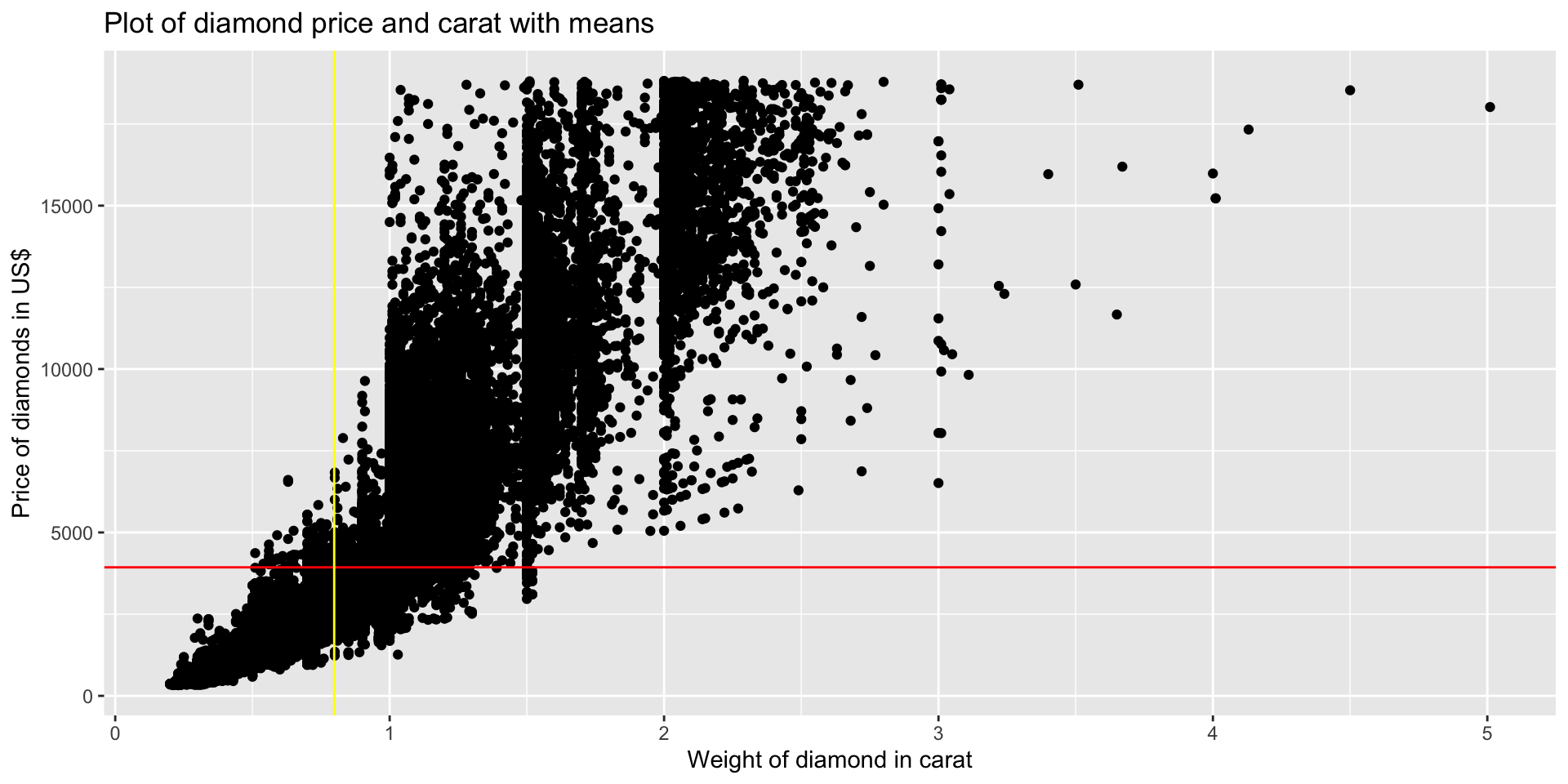
Price vs carat

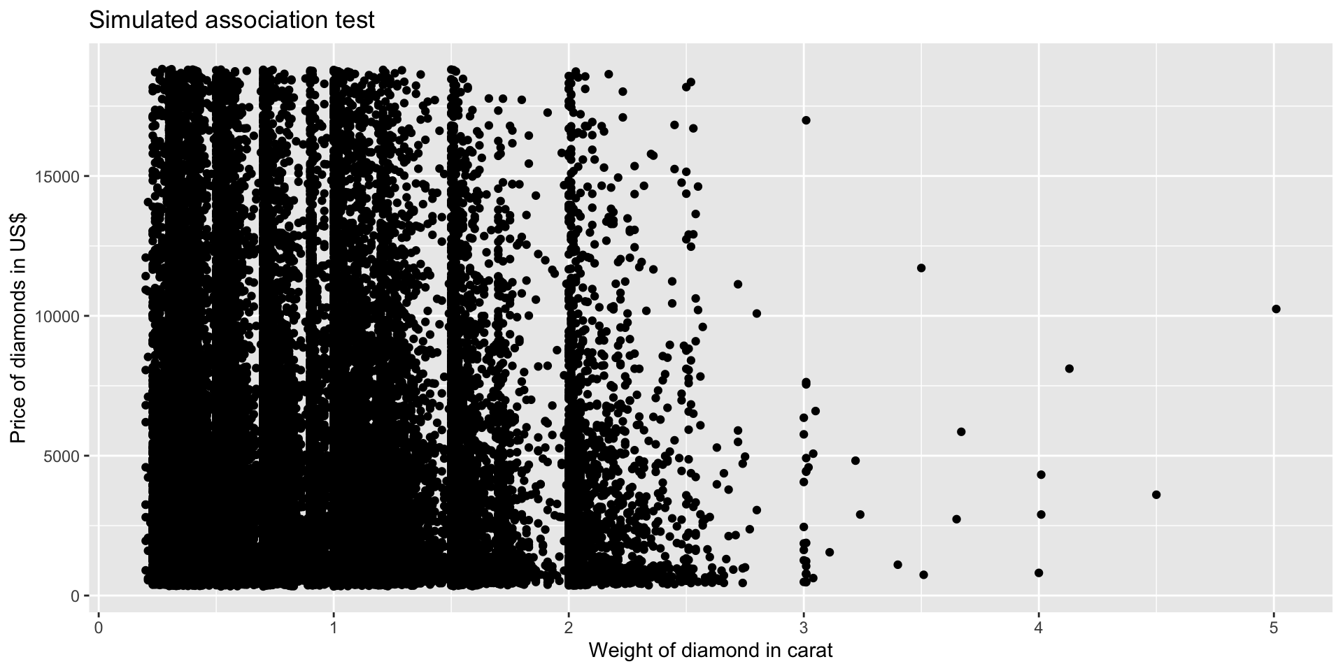
Visual association test

Ask them to run the coding in RStudio and see what they get - can connect some of their computers to the big screen

Can they see a difference between their plots and the real plot? What is the difference?

diamonds %>% # filtered data
  slice_sample(n = nrow(.)) %>% # random sample rows
  pull(carat) %>% # take out the variable carat
  bind_cols(., diamonds$price) %>% # price in the same order and bound to carat in different order
  ggplot() + # into ggplot
  geom_point(aes(y = ...2, x = ...1)) + # using the new names
  labs(title = "Simulated association test", 
       x = "Weight of diamond in carat", 
       y = "Price of diamonds in US$")

Describing a scatter plot

What is the difference between the actual plot and the simulated plots?

Discuss each point.

Big words make you sound smart to people that aren’t that smart.

• Trend or direction
  • positive
  • negative
• Curvature
  • linear
  • nonlinear
    • exponential
    • quadratic

• Variation
  • homoscedasticity (similar variance)
  • heteroscedasticity (different variance)
• Outliers
  • any weird points (explore these)
• Groupings

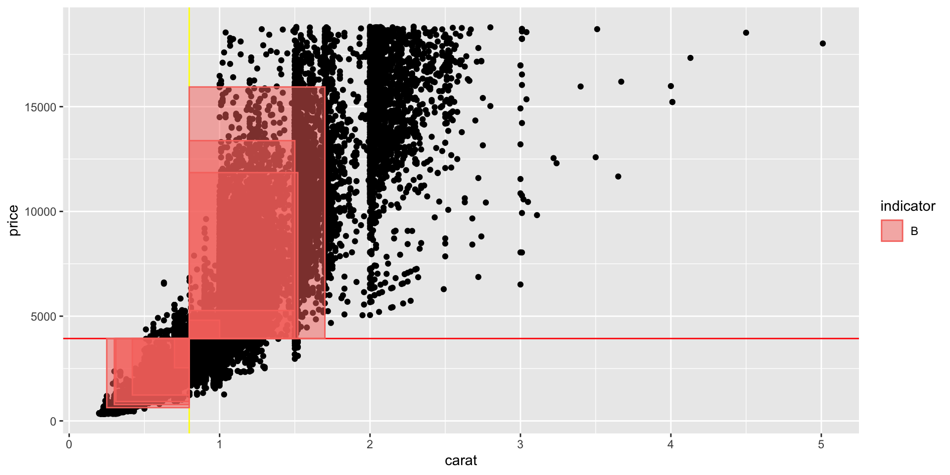
Describe these plots

What are the relationships between each plot?

What do the numbers mean?

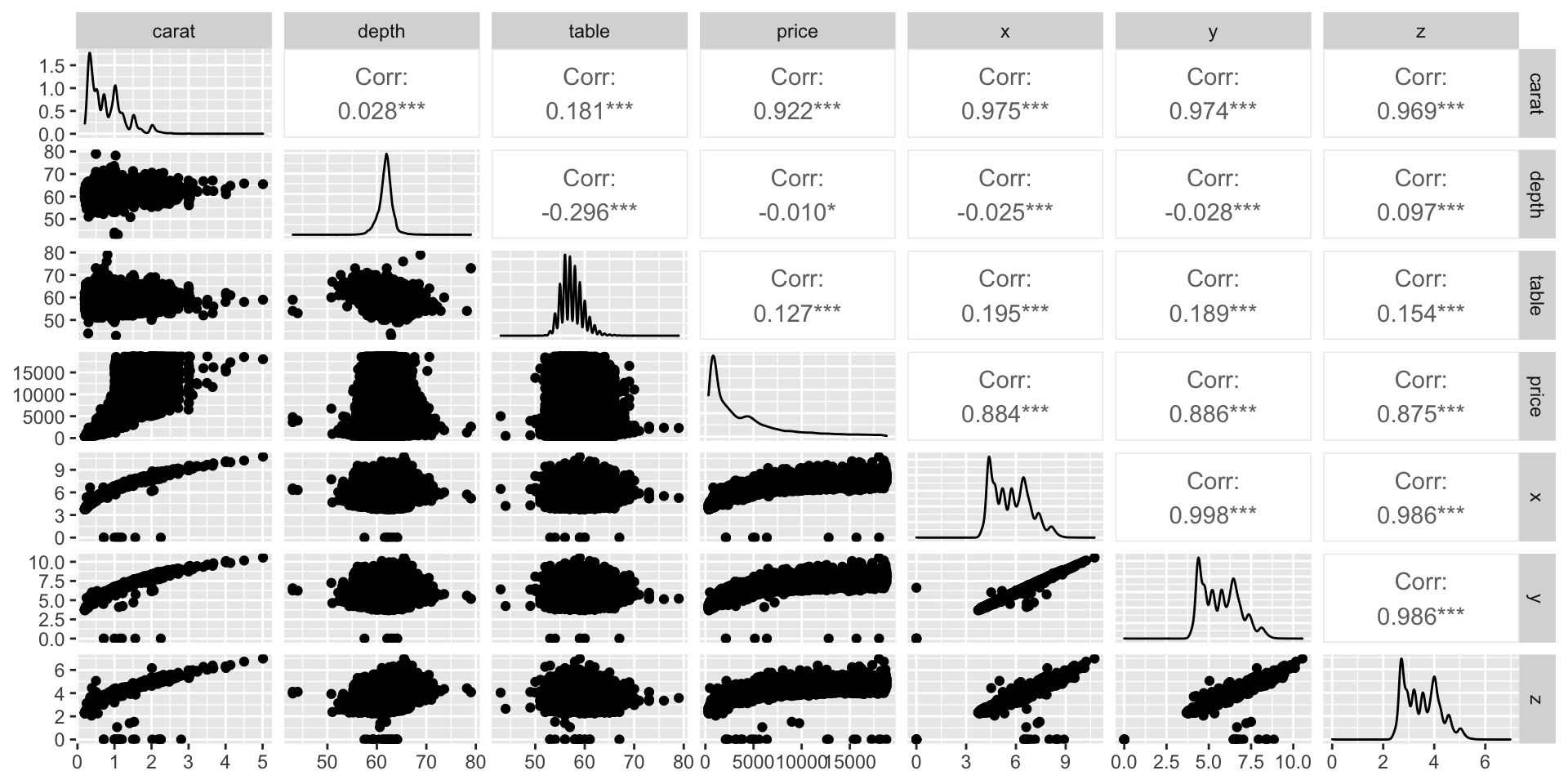
Measuring association

How can we quantify this stuff?

Measuring association

Remind them of the variance and what we did with the squares. What squares could we use now?

Covariance

If the product is negative then there it contributes to a negative trend - downhill from left to right.

Same if positive

hard to get ones that are negative for this dataset b/c tbere is a really strong positive association

Covariance math

This is a measure of the squares. We’d like a measure that is one dimensional. We want to look at more than just squares.

\(cov(x, y) = \frac{(x_1 - \bar{x})(y_1 - \bar{y}) + (x_2 - \bar{x})(y_2 - \bar{y}) + \ldots + (x_n - \bar{x})(y_n - \bar{y})}{n-1}\)

Correlation math

Standardizes the strength of the association

\[corr(x, y) = \frac{cov(x, y)}{s_x \cdot s_y}\]

Correlation characteristics

Standardizes the strength of the association

1. Referred to as \(r\)
2. Strength of linear association
3. \(r\) is always between \(-1\) and \(+1\), \(-1 \leq r \leq 1\).
4. \(r\) does not have units

Computing in R

Standardizes the strength of the association

# covariance of price and carat
cov(diamonds$price, diamonds$carat)

[1] 1742.765

# correlation of price and carat
cor(diamonds$price, diamonds$carat)

[1] 0.9215913

# coding for the pairs plots
# library(GGally)
# diamonds %>% # dataset
#  select_if(is.numeric) %>% # numeric variables
#  filter(y < 20, # y less than 20
#         z < 20, # z less than 20
#         table < 90) %>% # table less than 90
#  ggpairs(.) # make the plot

Line of association

What do these numbers mean?

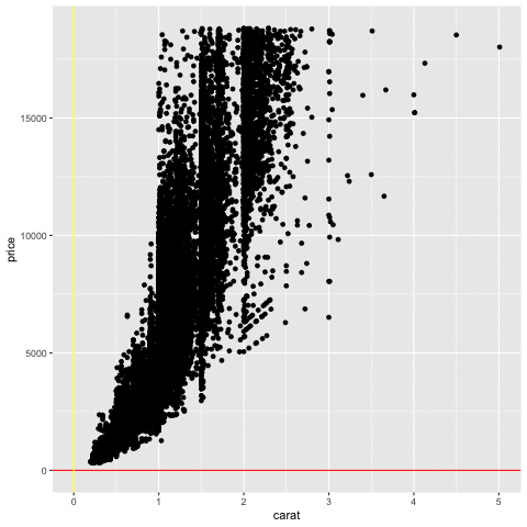
\[ y = mx + b \]

• \(m\) is gradient \(b\) is the \(y\) intercept

Gradient and slope

Pull out your calculators and work on this

\[ m = \frac{r \cdot s_y}{s_x} \] \[ b = \bar{y} - m \bar{x} \]

Fitting by hand

• \(r = 0.9215913\)

• \(s_{price} = 3989.44\)

• \(s_{carat} = 0.4740112\)

• \(m = \frac{r \cdot s_{price}}{s_{carat}}\)

• \[\begin{aligned} m &= \frac{r \cdot s_{price}}{s_{carat}} \\ &= \frac{0.9215913 \cdot 3989.44}{0.4740112} \\ &= 7756.426 \end{aligned}\]

Fitting by hand

• \(b = \overline{price} - m \cdot \overline{carat}\)

• \(\overline{price} = 3932.8\)

• \(\overline{carat} = 0.7979397\)

• \(m = 7756.426\)

• \[\begin{aligned} b &= \overline{price} - m \cdot \overline{carat} \\ &= 3932.8 - 7756.426 \cdot 0.7979397\\ &= -2256.36 \end{aligned}\]

• Our model is: \(\widehat{\text{price}} = -2256.36 + 7756.426 \cdot \text{carat}\)

Prediction by hand

Pull out your calculators and work on this

for carat values \(2.5\)

• \(\widehat{\text{price}} = -2256.36 + 7756.426 \cdot \text{carat}\)

• \[\begin{aligned} \widehat{\text{price}} &= -2256.36 + 7756.426 \cdot \text{carat} \\ &= -2256.36 + 7756.426 \cdot 2.5 \\ &= \$17135 \end{aligned}\]

Fit & predict in R

first use of tidymodels package

# library tidymodels
library(tidymodels)

## Assign the least
## squares line
least_squares_fit <- 
  linear_reg() %>% 
  set_engine("lm") %>% 
  fit(price ~ carat, data = diamonds) 
## NOTE: outcome first, predictor second

## Find the prediction
predict(least_squares_fit, tibble(carat = c(1, 2, 2.5, 4)))

# A tibble: 4 × 1
   .pred
   <dbl>
1  5500.
2 13256.
3 17135.
4 28769.

Warnings

• ALWAYS draw plots first
• numeric variables
• Linear relationship
• Check for outliers
• Lurking variables

Spurious correlations

• 100% of people who eat ketchup die
• amount of sunscreen used and probability of getting skin cancer
• birth order and probability of down syndrome
• countries with more smokers also have higher life expectancy
• More shark attacks are associated with higher levels of ice cream sales.
• The more volunteers at a natural disaster, the more destruction

More spurious correlations

• These variables are called lurking variables or confounders.

• Lurking variables are not considered in the statistical analysis

• Confounders are considered

• There are both known and unknown confounders, uknown confounders are lurking variables.

Click here for more spurious correlations

Your turn

Click here or the qr code below