Chapter 12: The normal probability model

STAT 1010 - Fall 2022

Learning outcomes

• The shape of the normal distribution and why it is important
• The central limit theorem.
• Understand shift and scales and how to compute them to find \(z\) scores
• Basic tests of normality including qqplots and kurtosis

Binomial -> Normal

As the number of trials increases, the binomial pdf becomes well approximated by a normal distribution.

“Observed data often represent the accumulation of many small factors.”

Normal

\(Y \sim N(\mu = 4, \sigma^2 = 25)\)

• We use two parameters to describe a Normal distribution
• \(Y \sim N(\mu = 0, \sigma^2 = 1)\)
• \(Y\) above is the standard normal distribution

Central limit theorem

There are multiple versions of the CLT

The probability distribution of a sum of independent random variables of comparable variance approaches a normal distribution as the number of summed random variables increases.

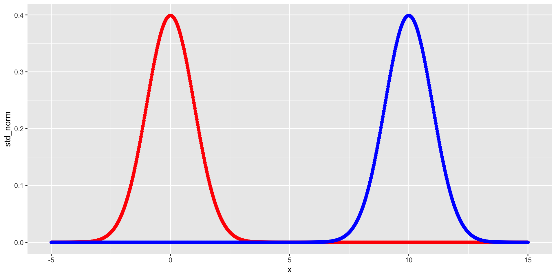
Shifts & scales

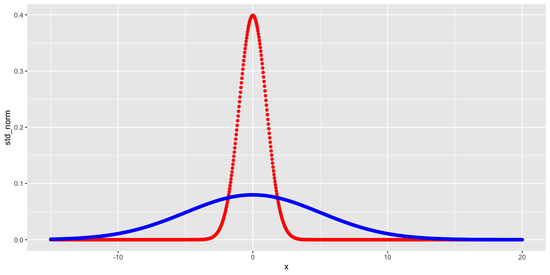
Standardizing

Books and tables of just normal probabilities to multiple decimal places.

Historically, it could be quite hard to find probabilities, so standardizing was important.

• use shift and scale information from above
• \(Z = \frac{X-\mu_X}{\sigma_X}\)
• Find \(E(Z)\)
• \(E(Z) = E(\frac{X-\mu_X}{\sigma_X})\)
• \[\begin{aligned} E(Z) & = E(\frac{X-\mu_X}{\sigma_X})\\ & = \frac{1}{\sigma_X}E(X-\mu_X) \\ &= 0 \end{aligned}\]

02:00

Standardizing

• use shift and scale information from above
• \(Z = \frac{X-\mu_X}{\sigma_X}\)
• Find \(Var(Z)\)
• \[\begin{aligned} Var(Z) & = Var(\frac{X-\mu_X}{\sigma_X})\\ & = \frac{1}{\sigma^2}Var(X-\mu_X) \\ &= \frac{\sigma^2}{\sigma^2} = 1 \end{aligned}\]

02:00

Example

Let \(Y \sim N(\mu_Y = 5, \sigma_Y^2 = 4)\), standardize the following and find the probability:

• \(P(Y < 3)\)

• \[\begin{aligned} P(Y < 3) &= P(\frac{Y - \mu_Y}{\sigma_Y} < \frac{3-\mu_Y}{\sigma_Y}) \\ & = P(Z < \frac{3-5}{2} = -1) \end{aligned}\]

• pnorm(-1) \(0.1586553\)

• pnorm(-1, mean = 5, sd = 2)

02:00

Queen Bee

To the left, to the left, pnorm is to the left

Percentiles are always to the left.

Example

Both of these probabilities are the same because of symmetry of the normal distribution. How does this generalize to all normal distributions?

Let \(Y \sim N(\mu_Y = 5, \sigma_Y^2 = 4)\), standardize the following and find the probability:

• \(P(Y > 7)\)

• \[\begin{aligned} P(Y > 7) &= P(\frac{Y - \mu_Y}{\sigma_Y} > \frac{7-\mu_Y}{\sigma_Y}) \\ & = P(Z > \frac{7-5}{2} = 1) \end{aligned}\]

• pnorm(1) \(0.8413447\)

• pnorm(1, mean = 5, sd = 2)

02:00

Graph

Example (cont’d)

This and the previous example have the same probabilities attached to them b/c the distribution is symmetric

Since they generally have the same shape what other things are true?

• \(P(Z > 1) = 1 - P(Z<1)\)
• 1 - pnorm(1) \(0.1586553\)
• 1 - pnorm(1, mean = 5, sd = 2)

02:00

Rule

This is true of all normal distributions, point of inflection, other things.

We will also need to learn to undo things. If we have a probability go backwards and find the z-score.

Undo

Percentiles

Earlier we used the normal to find a percent, you can also use R to find the z value for a certain percent.

• Find \(z : P(Z < z) = .1711\)
• qnorm(.1711) \(-0.9498273\)
• A medical test produces a score that measures the risk of a disease. In healthy adults, the test score is normally distributed with \(\mu=10\) point and \(\sigma = 2.5\). Lower scores suggest the disease is present. Test scores below what threshold signal a problem for only \(1\%\) of healthy adults?
• qnorm(.01, mean = 10, sd = 2.5) \(4.18413\)

02:00

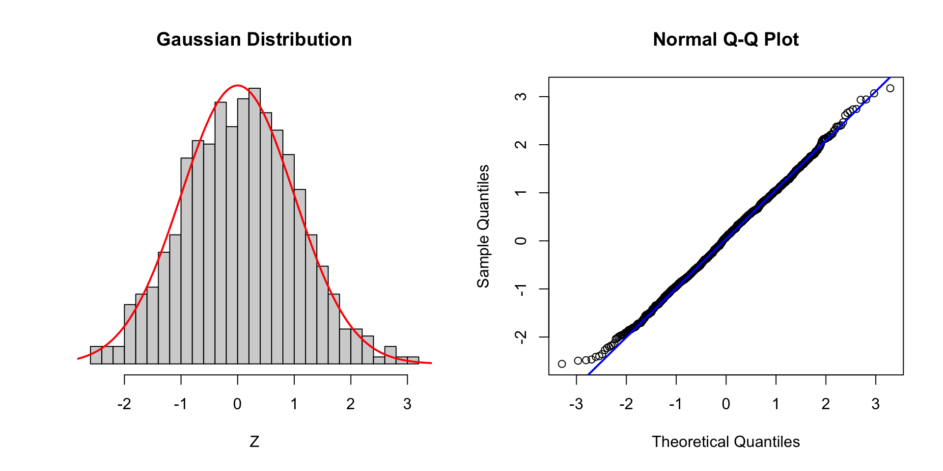
Normality tests

Looking at the data

• multimodal
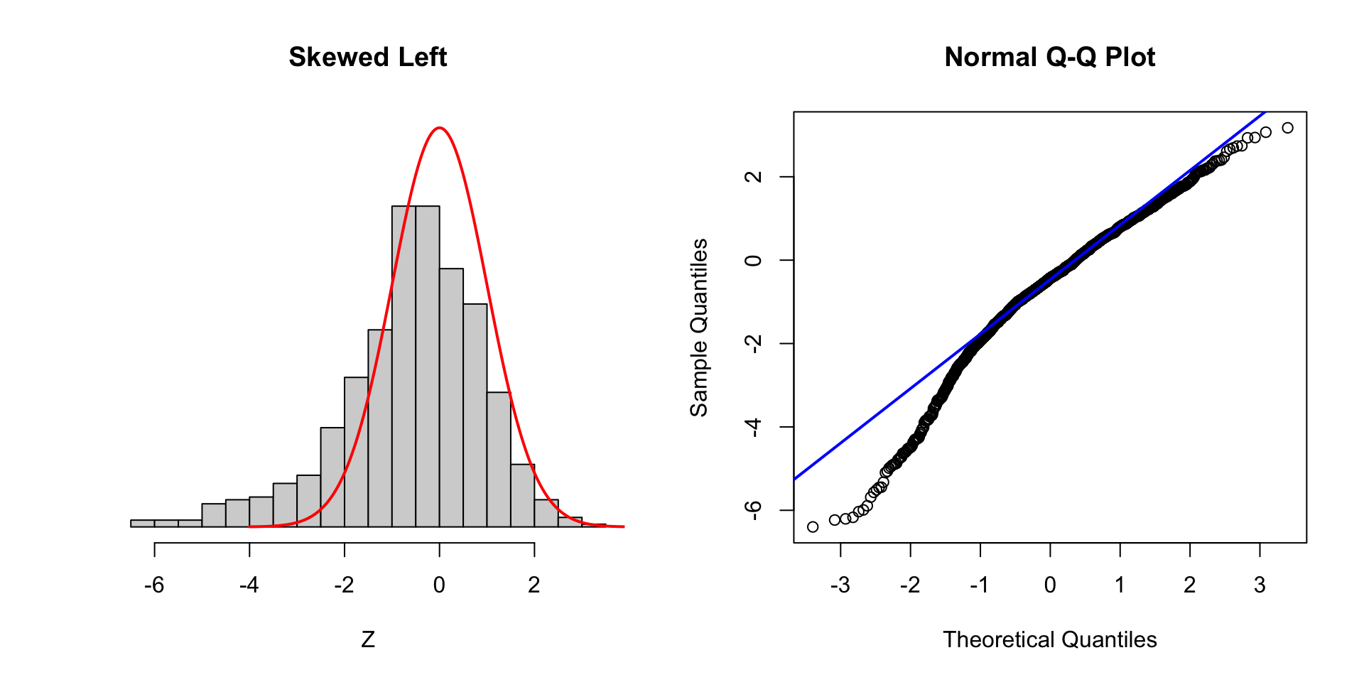
• skewness
• outliers

Plot - normal

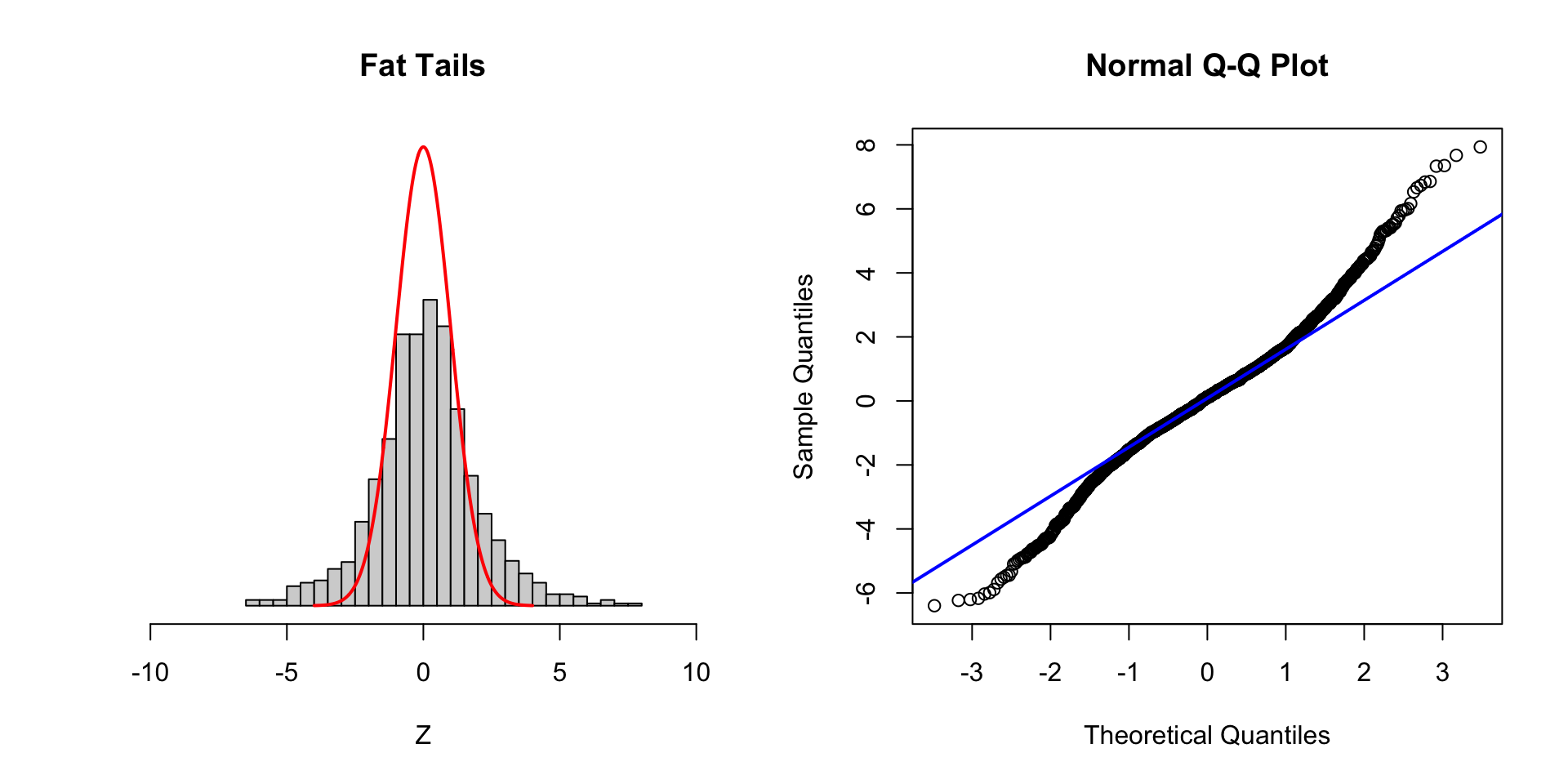
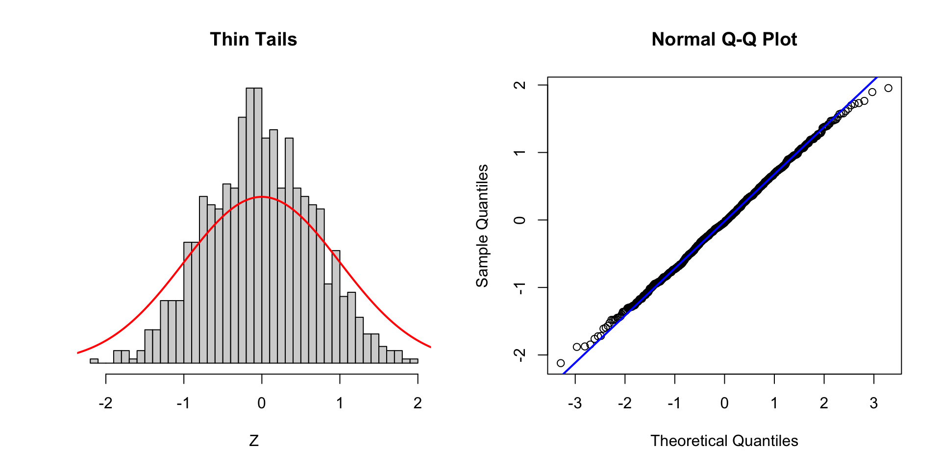
Plot - tale of 2 tails

Tale of 2 tails

Fat tails

Thin tails

Bimodal

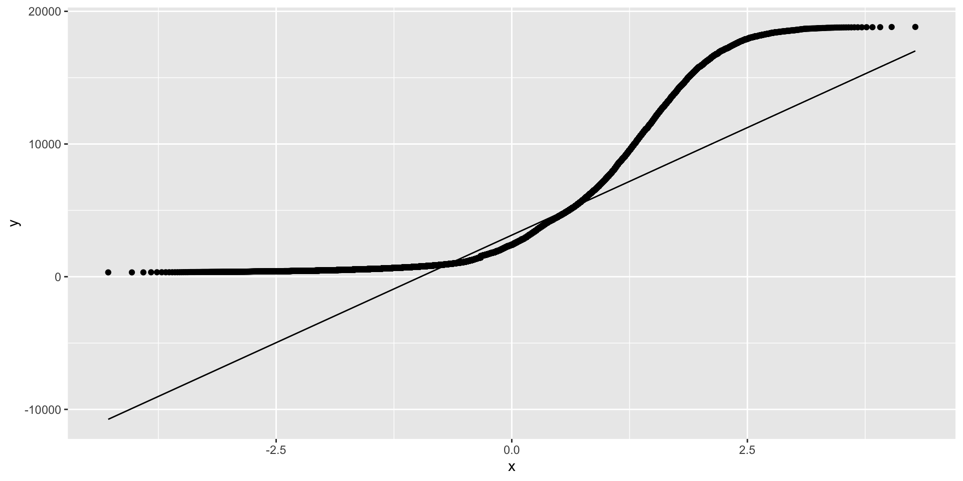
QQPlot in R

ggplot(diamonds, aes(sample=price)) +
  stat_qq() + # add the dots
  stat_qq_line() # and the line

Skewness

• find the \(z\) scores for all data (\(z_i = \frac{x_i - \bar{x}}{s}\))
• \[K_3 = \frac{z_1^3 +z_2^3 + ... + z_n^3}{n}\]
• If \(K_3 \approx 0\), then \(x\) is symmetric
• As \(K_3\) gets larger than 0, more right-skewed
• As \(K_3\) gets smaller than 0, more left-skewed

Kurtosis

• find the \(z\) scores for all data (\(z_i = \frac{x_i - \bar{x}}{s}\))
• \[K_4 = \frac{z_1^4 +z_2^4 + ... + z_n^4}{n} - 3\]
• If \(K_4 \approx 0\), then \(x\) is approximately normal
• As \(K_4 < 0\) flat uniform distribution without tails
• As \(K_4 > 0\) many outliers

Take home

If you see departures from normality (large or small kurtosis, QQ plots that deviate from a straight line) PLOT the data and check.