Chapter 15: Confidence intervals

STAT 1010 - Fall 2022

Learning outcomes

Building confidence intervals for the population proportion
Building confidence intervals for the population mean
Understanding the $t$ distributions
Interpreting confidence intervals
Understand the margin of error and how to use it to compute sample sizes

Revision

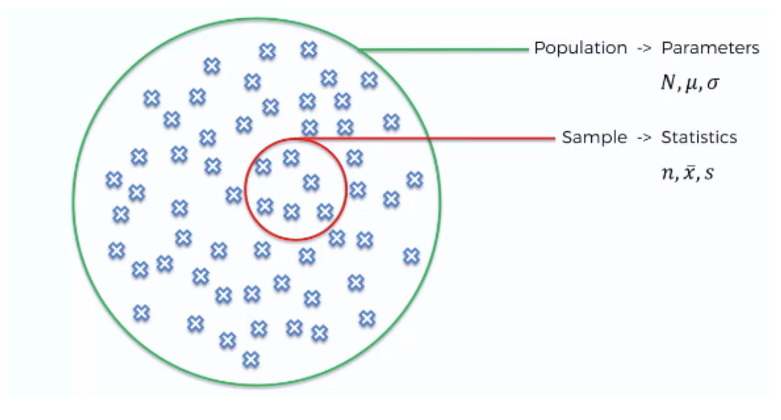
Confidence interval for proportion

What percent of customers are pleased with your service?
What percent of customers will refinance their loans?
What percentage of employees are in favor of a uniform change?
What percentage of voters will vote for Fetterman?

Variability

dependent on $p$ - fatter in middle, skinnier near 0 and 1
dependent on $n$, number of samples, bigger sample, less variability

Variability - math

\[ \hat{p} \sim N(\mu = p, \sigma^2 = \frac{p(1-p)}{n}) \]

numerator of the variance is similar to that of a Binomial distribution
as sample size increases, variance decreases

CI - math

\[\hat{p} \pm z_{\alpha/2} \cdot \sqrt{\hat{p}(1-\hat{p})/n} \] For $95\%$ CI, $z_{\alpha/2} = 1.96$

As confidence level increases, interval widens

In R: qnorm(0.025)

Assumptions

SRS condition The observed sample is SRS from the appropriate population. If population is finite, less than 10% of total population
Sample size condition (for proportion) both $n\hat{p}$ and $n(1-\hat{p})$ are larger than 10.

Example 1

Let $\hat{p}= 0.14$ and $n = 350$, find a $95\%$ CI for the proportion
$\begin{aligned} se(\hat{p}) &= \sqrt{\frac{\hat{p}(1-\hat{p})}{n}} &= \sqrt{\frac{0.14(1-0.14)}{350}}\end{aligned} \approx 0.0185$
lower value: $\hat{p} - 1.96 \cdot 0.0185 \approx 0.10374$
upper value: $\hat{p} + 1.96 \cdot 0.0185 \approx 0.17626$

Example 2

An auditor checks a sample of 225 randomly chosen transactions from among the thousands processed in an office. Thirty-five contains errors in crediting or debiting the appropriate account

a. Does this situation meet the conditions required for a $z$-interval for the proportion?

b. Find the $95\%$ confidence interval for $p$, the proportion of all transactions processed in the this office that have these errors.

c. Managers claim that the proportion of errors is about $10\%$. Does that seem reasonable?

Example 2 - solns

yes, $\hat{p} = 35/225 \approx 0.156$ so $n\hat{p}, n(1-\hat{p})> 10$ and we assume sampled $<10\%$
$\begin{aligned} \hat{p} \pm z_{\alpha/2} \cdot \sqrt{\hat{p}(1-\hat{p})/n} &= 0.156 \pm 1.96 \sqrt{0.156(1-0.156)/225}\\ &= 0.156 \pm 1.96 \cdot 0.0242 \\ &= 0.156 \pm 0.047\\ & [0.109, 0.203]\end{aligned}$
No $10\%$ is too low, with $95\%$ confidence it is higher

Confidence interval for mean

Average weight for filled ice cream containers
Average purchases from a website in US$

Variability

standard deviation of distribution
- higher sd -> wider CI
sample size
- smaller sample size -> wider CI

CI - mean

\[\bar{x} \pm t_{\alpha/2, n-1} \cdot \frac{s}{\sqrt{n}} \]

T - distribution

$Z = \frac{X-\mu_X}{\sigma_X}$
$\bar{X} \sim N(\mu = \mu\_X, \sigma^2 = \frac{\sigma_X^2}{n})$
$T_{n-1} = \frac{\bar{X}-\mu_X}{S/\sqrt{n}}$
$t$ distribution has more density in the tails to account for smaller sample sizes

Variability

dependent on $confidence \text{ }level$ - as confidence level increases so does the width of the interval
dependent on $n$, number of samples, bigger sample, less variability

Assumptions

SRS condition The observed sample is SRS from the appropriate population. If population is finite, less than 10% of total population
Sample size condition the sample size is larger than 10 times the absolute value of the kurtosis, $n>10|K_4|$.

Example 1

Let $\bar{x}= \$3285$, $n = 150$, and $s = \$238$ find a $95\%$ CI for the mean
$\begin{aligned} se(\bar{x}) &= s/\sqrt{n} &= 238/\sqrt{150}\end{aligned} \approx 19.43262$
qt(.025, df = 149) $\approx -1.976$
lower value: $3285 - 1.976 \cdot 19.43262 \approx \$3,320$
upper value: $3285 + 1.976 \cdot 19.43262 \approx \$3,247$
3285 + qt(.025, df = 149)* 238/sqrt(150)

Example 2

Office administrators claim that the average amount on a purchase order is $6,000. A SRS of 49 purchase orders averages $\bar{x} = \$4,200$ with $s = \$3,500$.

What is the relevant sampling distribution?
Find the 95% confidence interval for $\mu$, the mean of purchase orders handled by this office during the sampling period.
Do you think the administrators claim is reasonable?

Example 2 - solns

$N(\mu, \sigma^2/49)$
\[\begin{aligned} 4200 \pm 2.01 \cdot 3500/\sqrt{49} &= 4200 \pm 2.01 \cdot 500 \\ &= 4200 \pm -1005.317 \\ &\approx [3195, 5205]\end{aligned}\]
No $\$6,00$ is way above the $95\%$ confidence interval

Interpreting CI

“We can be 95% confident that the average purchase order handled by this office lies between $3195 and $5205.”

Manipulating CI

In example from means. How could we update the CI if we know we had 10 offices with similar purchase patterns.

If $[L \text{ to } U]$ is a $100(1 – \alpha)%$ confidence interval for $\mu$
then $[c \cdot L \text{ to } c \cdot U]$ is a $100 (1 – \alpha)%$ confidence interval for $c \cdot \mu$
and $[c + L \text{ to } c + U]$ is a $100(1 – \alpha)%$ confidence interval for $c + \mu$.

Example 2 - solns

$10 \cdot [3195, 5205] = [31950, 52050]$

Margin of error

\[\bar{x} \pm \frac{2s}{\sqrt{n}} \]

Margin of error = $\frac{2s}{\sqrt{n}}$

Sample size - mean

\[n = \frac{4s^2}{\text{(Margin of error)}^2} \]

For $p$ use $p = 0.5$ for biggest variance

Your turn

Click here or the qr code below