Chapter 19: Linear patterns

STAT 1010 - Fall 2022

Learning outcomes

Identify and graph the response and explanatory variable associate with a linear regression equation
Interpret the intercept and slope that define a linear regression
Summarize the precision of a fitted regression equation using the $r^2$ statistic and standard deviation of the residuals
Use residuals from the regression equation to check that the equation is an appropriate summary of the data

Reminders

We have fit a line to data already. Today we will discuss this in more detail.

For the diamonds dataset:

Which variable would we want to predict?
Which variable is a good predictor for it?

Variable names

variable on the $y$ axis
- dependent
- response
- outcome
variable on the $x$ axis
- independent (not this kind of independence)
- explanatory
- predictor

Plot the data

Fit

\[ \hat{y} = b_0 + b_1\cdot x \]

$b_1$ is gradient $b_0$ is the $y$ intercept
$\hat{y}$ is the fitted value, the result of the fitted line

Possible fits

Least squares

Gradient and slope

\[ b_1 = \frac{r \cdot s_y}{s_x} \] \[ b_0 = \bar{y} - b_1 \bar{x} \]

Example 1

$r = 0.9215913$
$s_{price} = 3989.44$
$s_{carat} = 0.4740112$
$b_1 = \frac{r \cdot s_{price}}{s_{carat}}$
$\begin{aligned} b_1 &= \frac{r \cdot s_{price}}{s_{carat}} \\ &= \frac{0.9215913 \cdot 3989.44}{0.4740112} \\ &= 7756.426 \end{aligned}$

Example 1

$b_0 = \overline{price} - b_1 \cdot \overline{carat}$
$\overline{price} = 3932.8$
$\overline{carat} = 0.7979397$
$b_1 = 7756.426$
\[\begin{aligned} b_0 &= \overline{price} - b_1 \cdot \overline{carat} \\ &= 3932.8 - 7756.426 \cdot 0.7979397\\ &= -2256.36 \end{aligned}\]
Our model is: $\widehat{\text{price}} = -2256.36 + 7756.426 \cdot \text{carat}$

Example 1

for carat values $2.5$

$\widehat{\text{price}} = -2256.36 + 7756.426 \cdot \text{carat}$
$\hat{y} = -2256.36 + 7756.426 \cdot x$
$\begin{aligned}\hat{y} &= -2256.36 + 7756.426 \cdot x \\ &= -2256.36 + 7756.426 \cdot 2.5 \\&= \$17135 \end{aligned}$

Residuals

The residual for the $i^{th}$ observation is \[ \begin{aligned} e_i &= y_i - \hat{y_i} \\ &= y_i - b_0 - b_1 \cdot x_i \end{aligned}\]

The sum of squared residuals is

\[e^2_1 + e^2_2 + \dots + e^2_n\]

The least squares line is the one that minimizes the sum of squared residuals

Example 2

Find the residual for the pair $(2.5, 16955)$

\[ \begin{aligned} e &= y - \hat{y} \\ &= 16955 - (-2256.36 + 7756.426 \cdot 2.5) \\ &= 16955 - 17134.71\\ &= -179.705 \end{aligned}\]

In `R`

# for model fitting and to get residuals
library(tidymodels)


## Assign the least
## squares line
lm_fit<- lm(price ~ carat, diamonds) 
## NOTE: outcome first, predictor second

## find predictions and residuals
head(augment(lm_fit), 5)

# A tibble: 5 × 8
  price carat .fitted .resid      .hat .sigma     .cooksd .std.resid
  <int> <dbl>   <dbl>  <dbl>     <dbl>  <dbl>       <dbl>      <dbl>
1   326  0.23 -472.     798. 0.0000452  1549. 0.00000600       0.516
2   326  0.21 -628.     954. 0.0000471  1549. 0.00000892       0.616
3   327  0.23 -472.     799. 0.0000452  1549. 0.00000602       0.516
4   334  0.29   -7.00   341. 0.0000398  1549. 0.000000966      0.220
5   335  0.31  148.     187. 0.0000382  1549. 0.000000278      0.121

Interpretations

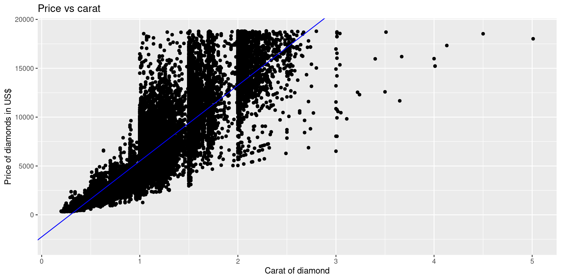
\[\widehat{\text{price}} = -2256.36 + 7756.426 \cdot \text{carat}\]

Intercept: For a diamonds that weighs 0 carats, we expect the price to be US$$-2256.36$.

Slope: For every 0.1 carat increase in diamond weight, we expect the price in $US to increase by 776, on average.

Visual interpretation

Extrapolation

This classic example is my favorite.

The model is only useful inside the values for which we have data. Outside of those values anything could happen.

Example 3

A manufacturing plant receives orders for customized mechanical parts. The orders vary in size, from about 30 to 130 units. After configuring the production line, a supervisor oversees the production. The least squares regression line that predicts time in hours using number of units to produce is:

\[\widehat{\text{time}} = 2.1 + 0.031 \cdot \text{Number of units}\] a. Interpret the intercept of the estimated line.

b. Interpret the slope of the estimated line.

c. Using the fitted line, estimate the amount of time needed for an order with 100 unit. Is this estimate an extrapolation?

d. Based on the fitted line, how much more time does an order with 100 units require over an order with 50 units?

Example 3 - solns

The intercept (2.1 hrs) is the estimated time for any orders, regardless of size (to set up production)
Once it is running, the estimated tiem for an order is 0.031 hours per unit (or 60 * 0.031 = 1.9 minutes)
$2.1 + 0.031\cdot 100 = 5.2 hours$, 100 units is inside the range
Fifty more units would need $0.031\cdot 50 = 1.55$ more hours

Properties of residuals

If the least squares line captures the association between $x$ and $y$, then a plot of residuals versus $x$ should stretch out horizontally with consistent vertical scatter.

In `R`

This plot has an obvious trend, the model does not fit the data well. We can use the visual association test to check.

## plotting residuals
augment(lm_fit) %>%
  ggplot() + 
  geom_point(aes(x = carat, 
                 y = .resid))

sd of residuals

If the residuals are nearly normal, we can summarise them with the mean and standard deviation.

\[ s_e = \sqrt{\frac{e_1^2 + e_2^2 + ... + e_n^2}{n-2}}\] the denominator is $n-2$ because we need two estimates for the line of best fit: $b_0$ and $b_1$.

Also known as RMSE root mean squared error. This can be used to compare multiple models to see which model best explains the variation in the data.

Explaining variation

A regression line splits the response into two parts, a fitted value and a residual

\[y = \hat{y} + e\] $\hat{y}$ represents the variation in $y$ that is associated with $x$ $e$ represents variation in $y$ due to other factors.

The sample correlation $0\leq r\leq 1$. The squared-correlation $r^2$ determines the fraction of the variation that can be accounted for by the model. $1-r^2$ is the amounted of variation left in the residuals.

In `R`

summary(lm_fit)


Call:
lm(formula = price ~ carat, data = diamonds)

Residuals:
     Min       1Q   Median       3Q      Max 
-18585.3   -804.8    -18.9    537.4  12731.7 

Coefficients:
            Estimate Std. Error t value Pr(>|t|)    
(Intercept) -2256.36      13.06  -172.8   <2e-16 ***
carat        7756.43      14.07   551.4   <2e-16 ***
---
Signif. codes:  0 '***' 0.001 '**' 0.01 '*' 0.05 '.' 0.1 ' ' 1

Residual standard error: 1549 on 53938 degrees of freedom
Multiple R-squared:  0.8493,    Adjusted R-squared:  0.8493 
F-statistic: 3.041e+05 on 1 and 53938 DF,  p-value: < 2.2e-16

Conditions

No obvious lurking variable: need to think about whether other explanatory variables might better explain the linear association between x and y.
Linear: use scatterplot to see if pattern resembles a straight line.
Random residual variation: use the residual plot to make sure no pattern exists.

Chapter 19: Linear patterns

Learning outcomes

Reminders

Variable names

Plot the data

Fit

Possible fits

Least squares

Gradient and slope

Example 1

Example 1

Example 1

Residuals

Example 2

In R

Interpretations

Visual interpretation

Extrapolation

Example 3

Example 3 - solns

Properties of residuals

In R

sd of residuals

Explaining variation

In R

Conditions

In `R`

In `R`

In `R`