| gender | happy | meh | sad |
|---|---|---|---|
| female | 100 | 30 | 110 |
| male | 70 | 32 | 120 |
Chapter 18: Inference for counts
STAT 1010 - Fall 2022
Learning outcomes
- Test for independence in a contigency table using a chi-squared test
- Check for a goodness of fit of a probability model using a chi-square test
- Find the appropriate degrees of freedom for a chi-squared test.
- Explain the similarities and differences between chi-squared tests and methods that compare two proportions
- Determine the statistical significance of a chi-squared statistic from
R
Revision
We have discussed this before and now we will formalize this work. Like walking up a lighthouse.
Test of independence
\[H_0: \text{Qualitative variable 1 and Qualitative variable 2 are independent}\]
\[H_A: \text{Qualitative variable 1 and Qualitative variable 2 are not independent}\]
Example 1
A manufacturing firm is considering a shift from a 5-day workweek (8 hours per day) to a 4-day workweek (10 hours per day). Samples of the preferences of 188 employees in two divisions produced the following contingency table:
Observed counts
| Divisions | ||||
|---|---|---|---|---|
| Clerical | Production | Total | ||
| Preferences | 5-day | 17 | 46 | 63 |
| 4-day | 28 | 38 | 66 | |
| Total | 45 | 84 | 129 |
a. What would it mean if the preference of employees is independent of division?
b. State \(H_0\) for the \(\chi^2\) test of independence in terms of the parameters of two segments of the population of employees.
Example 1 - solns
- Independence means that all the percent of people who prefer a 5-day work week is the same in all divisions. Lack of independence implies different percentages across divisions
- \(H_0: p_{clerical} = p_{production}\) \(H_A: \text{at least one of these differs}\)
Calculating \(\chi^2\)
If one variable is independent of the other, then the variable should have the same proportion in each level as the totals have in each level.
Expected counts
| Divisions | ||||
|---|---|---|---|---|
| Clerical | Production | Total | ||
| Preferences | 5-day | \(45/129\cdot63 \approx 22\) | \(84/129\cdot63 \approx 41\) | 63 |
| 4-day | \(45/129\cdot66 \approx 23\) | \(84/129\cdot66 \approx 43\) | 66 | |
| Total | 45 | 84 | 129 |
Calculating \(\chi^2\)
\[ \chi^2 = sum\frac{(observed - expected)^2}{expected}\]
We want to know how much this varies from the expected that is why the expected is the denominator.
Example 2
Find the expected counts for the following observed variables
Example 2 - solns
| happy | meh | sad |
|---|---|---|
| 88.31169 | 32.20779 | 119.4805 |
| 81.68831 | 29.79221 | 110.5195 |
Plot
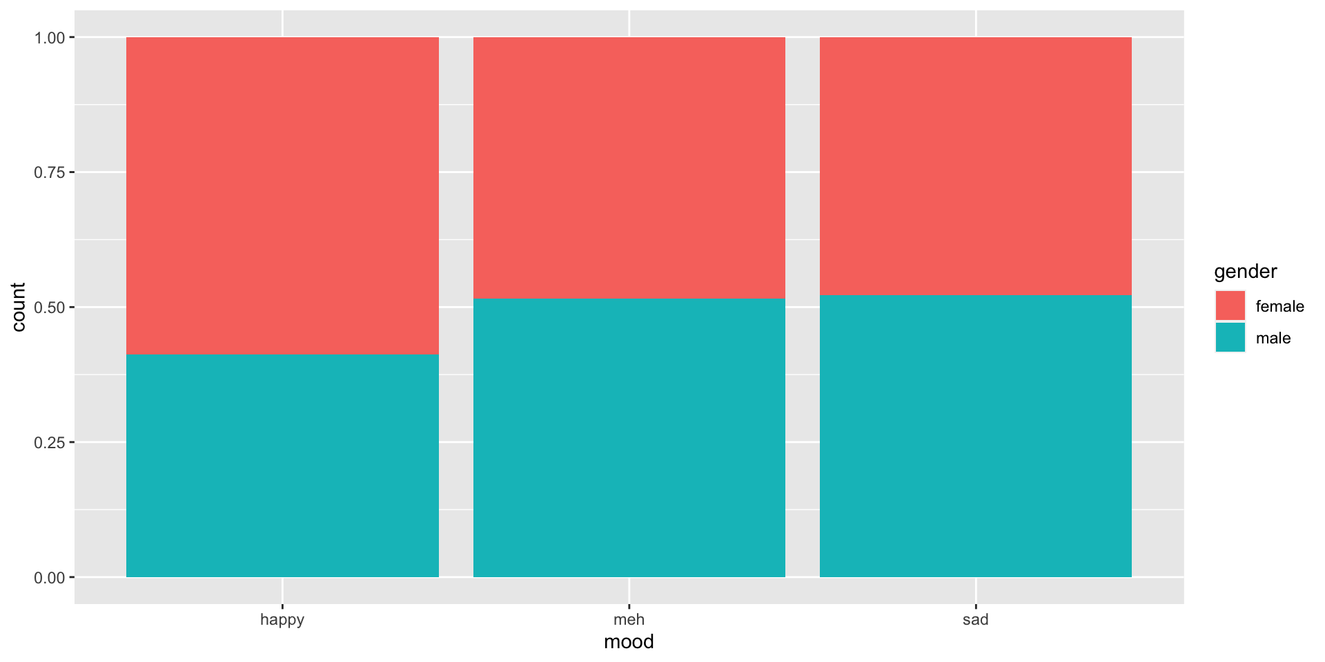
Reading plots
If the color change in the bars are approximately at the same height in every level of the variable on the \(x\) axis, this is evidence against rejecting \(H_0\). We might be more inclined to think that \(H_0\) is true.
Assumptions
- No lurking variables
- Data is a random sample from the population
- Categories must be mutually exclusive
- Each cell count must be at least 5 or 10 (more here)
degrees of freedom
\[df \text{ for a } \chi^2 \text{ test of independence} = (r-1)(c-1)\]
where \(r= \text{number of rows}\) and \(c= \text{number of columns}\)
Assumptions:
- Each cell count ideally 10, or 5 if the test has 4 or more degrees of freedom.
In R
- Find the totals
- Compute the expected counts
- Calculate \(\chi^2 = sum\frac{(observed - expected)^2}{expected}\)
- Find the df \((r-1)(c-1)\)
- Solve for the p-value
1 - pchisq(chi-square, df)
Example 3
In example 2, perform a hypothesis test and find the \(\chi^2\) value and the p-value. Are gender and mood independent?
Steps for a hypothesis test
- State hypotheses
- Determine the level of significance
- Check conditions
- Calculate test statistic
- Compute p-value
- Generic conclusion
- Interpret in context
Example 3 - solns
- \(H_0: p_h = p_m = p_s\) and \(H_A: \text{at least one differs}\)
- \(\alpha = 0.05\)
- Yes.
- \(\begin{aligned} \chi^2 &= sum\frac{(observed - expected)^2}{expected} \\ &= \frac{(100-88.3)^2}{88.3} + \frac{(70-81.7)^2}{81.7} + ... + \frac{(120-119.5)^2}{119.5}\\ &\approx 5.0999\end{aligned}\) \(df = (3-1)\cdot(2-1)\)
Example 3 - solns
1 - pchisq(5.099, df = 2)\(\approx 0.078\)- We fail to reject \(H_0\)
- We do not have evidence that gender and mood are associated, the data suggests they are independent.
Example 3 - solns
General vs Specific Hypothesis
The \(\chi^2\) test is a general test that provides evidence that one of the proportions might differ. To estimate which proportion differs we will need to build a confidence intervals like we did here.
Tests for randomness
There are a few places where \(\chi^2\) tests are particularly useful. For example, in fraud detection. Benford’s law outlines the frequency of first digits (1-9) in a number. If the proportions are significantly different than Benford’s law there may be evidence of fraud.
Test for goodness of fit
When an outcome is either Binomial or Poisson one way to check that predictions are correct is to perform a \(\chi^2\) test on the actual and predicted.
- A small p-value to indicates that these values are not independent.
Your turn
Click here or the qr code below